Transformers: My notes for developing an intuition
August 2, 2025
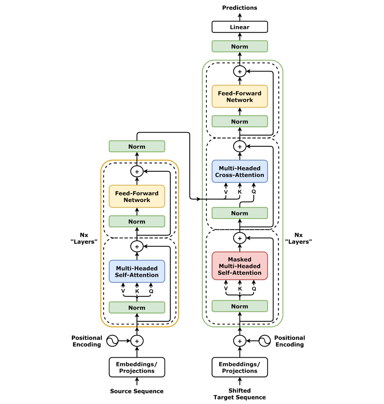
The Architecture
Note:
The original paper had layer normalization after the attention step, however a 2020 paper(arXiv:2002.04745) showed that normalization before attention stabilizes training, removing need for learning rate warmup. That change is represented here. In the original step they do "Layer Norm(\(X+Z(X)\))" the found-to-be-better approach does "\(X+Z(\text{LayerNorm}(X))\)"
- Tokenization: Inputs must be tokenized into their base properties
- A token can represent a character or a short segment of characters
- Example: He won't move -> He, won, ', t, move
- The exact way to tokenize the input depends on the implementation but typically we break up punctuation and complex words
- Embedding: Tokens are then embedded based on a one hot encoding of the token times an embedding matrix
- This result is a unique vector belonging to a n dimensional space. The embedding matrix is a learned matrix via another training proccess
- Positional Encoding: Embedding vectors are then mapped to a matrix by taking sin and cosine representations of the position to create a unique probability frequency representing the location of the embedding vector in the input.
- Alternates matrix frequencies by sin and cos to ensure uniqueness other position 1 and 6 in a space of 5 would have the same frequency
- Takes a 1xL embedding vector and creates a dxl, space where L is the length of the input and d is a determined positive even integer parameter
- d is a tunable parameter and often is the same as the word embedding dimension (for easier math), often 512, 768, or 1024 by your embedding function
- N is a parameter in positional encoding which should be significantly larger than the longest input you would expect
- By using matrixes, we allow for computationally simple matrix multiplication to go from one encoded position to another
- Encoder block: The matrix containing the positional encoding of the embedding vectors is the passed into the encoding block
- Layer normalization
- https://arxiv.org/abs/1607.06450
- In order to reduce training time and stabilize training we do a layer normalization on the original input matrix
- Layer Norm(X)
- Layer norm is just the z-score normalization with a small constant added to variance for numerical stability
- Multi head attention
- Links I used to understand
- Self-Attention mechanism intuition
- To find the relative importance of each word in comparison to one word in a sentence (toy example)
- We calculate the vector multiplication of word 1(q,1) across word 2 (through n, k\_1 to k\_n) to get a score
- \((q_1 \cdot k_i)\) for \(i=1, \dots, d_k\)
- We divide the scores by the square root of the sentence length (key vector dimension), this leads to more stable gradients
- \(\frac{q_1 \cdot k_i}{\sqrt{d_k}}\) for \(i=1, \dots, d_k\)
- We then take the SoftMax of each \(\frac{q_1 \cdot k_i}{\sqrt{d_k}}\), this gives us the relative importance of each word
- \(\text{Softmax}\left(\frac{q_1 \cdot k_i}{\sqrt{d_k}}\right)\) for \(i=1, \dots, d_k\)
- We then multiply each SoftMax value (relative importance of each word to first word) to our value vector (representation of original word vector), this maintains the representation of the words we want to focus on and minimizes the presence of the insignificant words
- \(v_i \cdot \text{Softmax}\left(\frac{q_1 \cdot k_i}{\sqrt{d_k}}\right)\) for \(i=1, \dots, d_k\)
- We then sum up our weighted value vectors, this produces the output of the self-attention layer, a vector representing the importance of each word in the sentence relative to a single word
- \(z_1 = \sum_{i=1}^{d_k} v_i \cdot \text{Softmax}_{v_i}\left(\frac{q_1 \cdot k_i}{\sqrt{d_k}}\right)\)
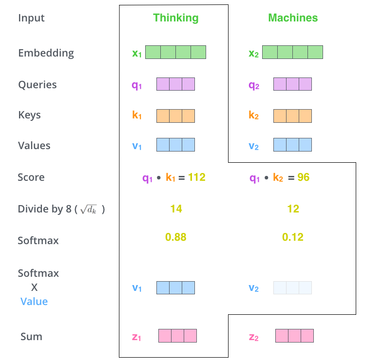
Image credit: Jay Alammar - We calculate the vector multiplication of word 1(q,1) across word 2 (through n, k\_1 to k\_n) to get a score
- In practice, this is done via matrixes for faster computations.
- Little fundamentally changes, as instead of individual z1 vectors we have a matrix z holding all z1 vectors
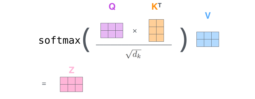
Image credit: Jay Alammar - To find the relative importance of each word in comparison to one word in a sentence (toy example)
- Multi-headed Self Attention mechanism intuition
- Multi-headed attention provides the model with a way to consider multiple positions at once, since often z1 is dominated by itself, allowing for multiple representation subspaces. Basically here's one opinion of the importance of each word, here's a second, and a third, and so on. When looking at a painting, we as humans each notice something unique, the multiple attention heads do the same
- This works by computing 'z' n times, in the original paper, it was 8. We randomly initiate our \(W_0^Q\), \(W_0^K\), \(W_0^V\) matrixes to allow for different gradients. When we have our 8 'Z' matrixes we then concatenate our matrixes and project them back to original dimension of Z. This is for the feed forward matrix which is expecting one matrix of dimensions Z
- Does so by concatenating our \(Z_0\) to \(Z_n\) matrixes then multiplying them by a \(W^O\) projection matrix to reduce it back to a single Z matrix rowsxcolumns
- This sums our attention heads 'opinions of relevance' to one opinion
- Add in original input
- The addition of the original input has been found to avoid vanishing gradient issues and stabilize the training process. So here we add in the normalized positional encoded embedding matrix to our attention output.
- X+Z(normalized X)
- (to add our opinion of relevance to our positional encoded input embedding)
- The addition of the original input has been found to avoid vanishing gradient issues and stabilize the training process. So here we add in the normalized positional encoded embedding matrix to our attention output.
- Layer normalization
- Feed forward
- https://aclanthology.org/2021.emnlp-main.446.pdf
- Intuitively this takes in inputted numerical representation and maps it to a latent representation space then the FNN acts as a key-value pair to produce a probability distribution over the vocabulary from the input
- The feedforward network is a 2-layered multilayer perceptron module of weights and bias vectors along an activation function \(FFN(x)=\sigma(xW_1+b_1)W_2+b_2\). The activation function originally was a ReLU activation function
- The number of neurons in the middle layer is typically larger (\~4 times) than the embedding size and is referred to as the intermediate or filter feedforward size
- Add in un-normalized data (post attention but pre second normalization)
- Into next encoder layer or decoder
- One last layer normalization
- Layer normalization
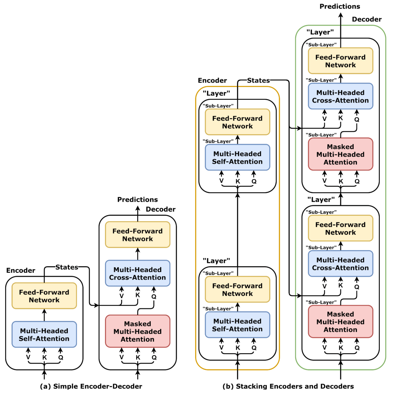
- Decoder block:
- Output embedding input
- The first encoder is either nothing or the previously outputted token, subsequent layers take the previous decoders output
- Normalize input
- Masked Multi-head Self Attention
- Same as other multi-head attention operation except here we set all future position values to be -inf, masking the values from consideration
- This intuitively considers what tokens are most relevant given what it has seen before
- Add original un-normalized input to attention output
- Layer normalization
- Encoder decoder Multi-head Cross Attention
- Here we initialize our K and V matrixes with the output of the encoders from before, Q is the output of the previous attention mechanism
- This draws relevant information from the encodings generated by the encoders
- Masking is not needed here as it attends to vectors computed before the decoder started decoding
- This intuitively considers which encoded latent knowledge spaces are most relevant to our normalized 'opinion of relevance' encoding
- Add in un-normalized data (post attention but pre second normalization)
- Layer Normalization
- Feed Forward
- Add in un-normalized data (post cross attention but pre third normalization)
- Into next decoder or linear SoftMax output
- Output embedding input
- Linear SoftMax layer:
- The output is un-embedded through a linear soft-max layer. Which turns the embedded vector into a probability vector over the vocabulary of tokens
- Linear layer
- A simple fully connected neural network that projects the decoder output into a much larger logits vector
- Intuitively this projects the output into a vector representing our entire vocabulary with an associated logit for each output
- SoftMax layer
- SoftMax takes this logit vector and turns it into a probability vector adding up to 1
- We then take the value with the highest probability and return the corresponding token (token since it could be a word or a punctuation)
How it is trained:
Usually first pre-trained on a large generic dataset using self-supervising learning. Then fine-tuned on a small task-specific dataset
Example loss functions are:
- Masked task: Correctly guessing a masked word in an input
- Autoregressive task: Entire sequence is masked, model produces an output for first token, output is revealed and error computed, does second token and so on
- prefixML task: Same as above but first half of sequence is immediately available.
- Translations between different languages, contexts, or modalities
- Judging linguistic and pragmatic acceptability of the language
All together:
Takes in an input and converts it to a vector, calculates the position of each token with respect to the entire input and adds the representation to the vector, then stores all the vectors as a matrix and passes it into the encoder or decoder.
The encoder takes the matrix, normalizes it, and finds the contextual relevance of each word with respect to each word; then adding this contextual importance back to the original matrix. The matrix is then normalized again and passed to a FFN which acts as key-value lookup of the matrix to the latent space returning a probability distribution over the vocabulary, which when added to our input begins the process of slowly converging on a result.
The decoder takes the input matrix representation, normalizes it, and finds the future-location-masked contextual relevance of each word with respect to each word; then adding this contextual importance back to the original matrix. The matrix is then normalized again and passed to a cross-attention system which takes in the learned encoder key and value matrixes to enrich our input with contextually relevant "information" from our latent knowledge space, this context is added back to our input. This matrix is then normalized again and passed to a FFN which acts as key-value lookup of the matrix to the latent space returning a probability distribution over the vocabulary, which when added to our input begins the process of slowly converging on a result.
Many layers later, the final matrix undergoes a linear transformation to logit representations across the vocabulary, then SoftMax returns probabilities of the logits. We then return the highest probability token.
The encoder process is repeated an incredible number of times minimizing various loss functions to create an incredibly rich and knowledgeable "brain" or latent representation of information that the decoder can pull from after training.
The decoder process is repeated until a terminal token is highest probability, whether through the models belief or via the models system prompt instructions.
Alternate implementation mechanics:
Different models use different:
- Activation functions
- Normalization algorithms
- Normalization locations
- Positional encodings
- Implementation efficiencies
- Alternate attention graphs
- Multimodal approaches
Links:
- https://peterbloem.nl/blog/transformers
- https://www.google.com/search?q=https://en.wikipedia.org/wiki/Transformer\_(deep\_learning\_architecture)\%23Subsequent\_work
- https://jalammar.github.io/illustrated-transformer/
- https://arxiv.org/abs/1607.06450
- https://aclanthology.org/2021.emnlp-main.446.pdf
- https://www.reddit.com/r/MachineLearning/comments/qidpqx/d\_how\_to\_truly\_understand\_attention\_mechanism\_in/